Calibrating Flow Cytometry Data to MEF
This tutorial focuses on how to transform flow cytometry data to Molecules of Equivalent Fluorophore (MEF) using FlowCal, particularly by using the module FlowCal.mef. For more information on MEF calibration, see the section on fundamentals of calibration.
To start, navigate to the examples directory included with FlowCal, and open a python session therein. Then, import FlowCal as with any other python module.
>>> import FlowCal
Also, import numpy and pyplot from matplotlib
>>> import numpy as np
>>> import matplotlib.pyplot as plt
Working with Calibration Beads
As mentioned in the fundamentals section, conversion to MEF requires measuring calibration beads. sample001.fcs in the FCFiles folder contains beads data. Let’s examine it.
>>> b = FlowCal.io.FCSData('FCFiles/sample001.fcs')
>>> b = FlowCal.transform.to_rfi(b)
>>> density_gate_output = FlowCal.gate.density2d(b,
...                                              channels=['FSC', 'SSC'],
...                                              gate_fraction=0.3,
...                                              full_output=True)
>>> b_g = density_gate_output.gated_data
>>> c   = density_gate_output.contour
>>> FlowCal.plot.density_and_hist(b,
...                               gated_data=b_g,
...                               gate_contour=c,
...                               density_channels=['FSC', 'SSC'],
...                               density_params={'mode':'scatter',
...                                               'xlim': [1e2, 1e3],
...                                               'ylim': [1e2, 1e3],
...                                               'sigma': 5.},
...                               hist_channels=['FL1'])
>>> plt.tight_layout()
>>> plt.show()
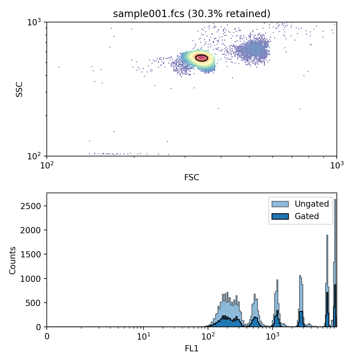
The FSC/SSC density plot shows two groups of events: the dense group in the middle corresponds to single beads, whereas the fainter cluster on the upper right corresponds to bead agglomerations. Only single beads should be used, so FlowCal.gate.density2d() is used here to identify single beads automatically. Looking at the FL1 histogram, we can clearly distinguish 8 subpopulations with different fluorescence levels. Note that the group with the highest fluorescence seems to be close to saturation.
MEF Transformation in FlowCal
We saw in the transformation tutorial that a transformation function is needed to convert flow cytometry data from raw sensor numbers, as stored in FCS files, to fluorescence values in a.u. Similarly, FlowCal uses transformation functions to convert these to MEF. However, these functions have to be generated during analysis using a calibration bead sample. Once a function is generated, though, it can be used to convert many cell samples to MEF, provided that beads and samples have been acquired using the same settings.
Generating a transformation function from calibration beads data is a complicated process, therefore FlowCal has an entire module dedicated to it: FlowCal.mef. The main function in this module, FlowCal.mef.get_transform_fxn(), requires at least the following information: calibration beads data, the names of the channels for which a MEF transformation function should be generated, and manufacturer-provided MEF values of each subpopulation for each channel. Let’s now use FlowCal.mef.get_transform_fxn() to obtain a transformation function.
>>> # Obtain transformation function
>>> # The following MEFL values were provided by the beads' manufacturer
>>> mefl_values = np.array([0, 792, 2079, 6588, 16471, 47497, 137049, 271647])
>>> to_mef = FlowCal.mef.get_transform_fxn(b_g,
...                                        mef_values=mefl_values,
...                                        mef_channels='FL1',
...                                        plot=True)
>>> plt.show()
The argument plot instructs FlowCal.mef.get_transform_fxn() to generate and save plots showing the individual steps of bead data analysis. We will look at these plots and how to interpret them in the next section. We recommend to always generate these plots to confirm that the standard curve was generated properly.
Let’s now use to_mef to transform fluroescence data to MEF.
>>> # Load sample
>>> s = FlowCal.io.FCSData('FCFiles/sample006.fcs')
>>>
>>> # Transform all channels to a.u., and then FL1 to MEF.
>>> s = FlowCal.transform.to_rfi(s)
>>> s = to_mef(s, channels='FL1')
>>>
>>> # Gate
>>> s_g = FlowCal.gate.high_low(s, channels=['FSC', 'SSC'])
>>> s_g = FlowCal.gate.density2d(s_g,
...                              channels=['FSC', 'SSC'],
...                              gate_fraction=0.5)
>>>
>>> # Plot histogram of transformed channel
>>> FlowCal.plot.hist1d(s_g, channel='FL1')
>>> plt.show()
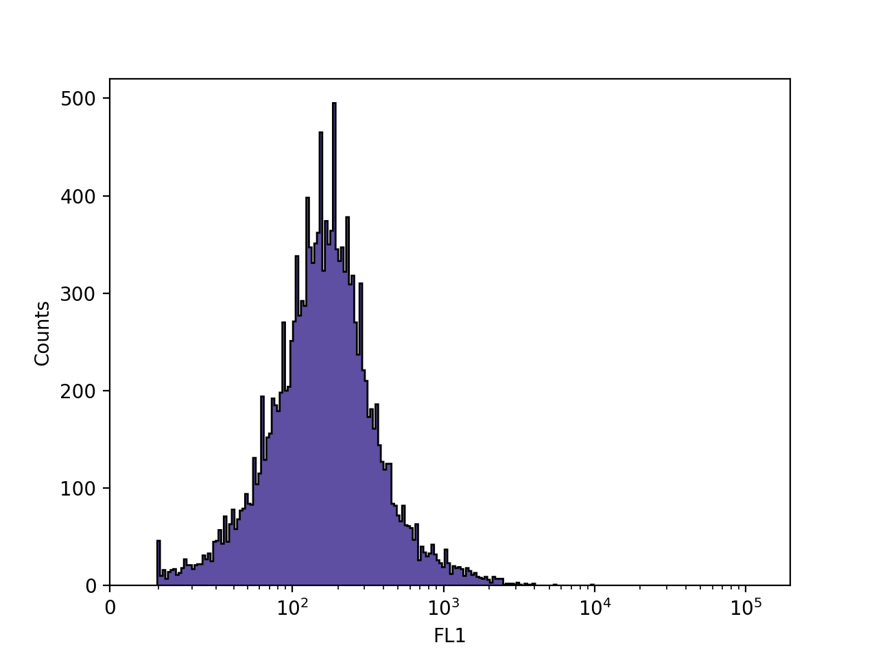
s_g now contains FL1 fluorescence values in MEF units. Note that the values in the x axis of the histogram do not match the ones showed before in channel (raw) units or a.u.. This is always true in general, because fluorescence is now expressed in different units.
Generation of a MEF Transformation Function
We will now give a short description of the process that FlowCal.mef.get_transform_fxn() uses to generate a transformation function from beads data. We will also examine the plots produced by FlowCal.mef.get_transform_fxn() and discuss how these plots can reveal problems with the analysis. In the following, <beads_filename> refers to the file name of the FSC cotaining beads data, which was provided to FlowCal.mef.get_transform_fxn(). This discussion is parallel to the one in the fundamentals of calibration document, but at a higher technical level.
Generating a MEF transformation function involves four steps:
1. Identification of Bead Subpopulations
FlowCal uses a clustering algorithm to automatically identify the different subpopulations of beads. The algorithm will try to find as many populations as values are provided in mef_values.
A plot with a default filename of clustering_<beads_filename>.png is generated by FlowCal.mef.get_transform_fxn() after the completion of this step. This plot is a histogram or scatter plot in which different subpopulations are shown in a different colors. Such plot is shown below, for sample001.fcs.
It is always visually clear which events correspond to which groups, and the different colors should correspond to this expectation. If they don’t, sometimes it helps to use a different set of fluorescence channels for clustering (see below), or to use a different gating fraction in the previous density gating step.
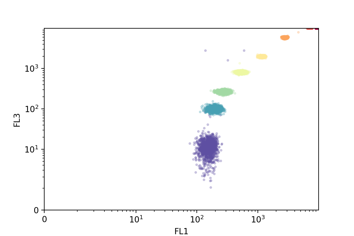
The default clustering algorithm is Gaussian Mixture Models, implemented in FlowCal.mef.clustering_gmm(). However, a function implementing another clustering algorithm can be provided to FlowCal.mef.get_transform_fxn() through the argument clustering_fxn. In addition, the argument clustering_channels specifies which channels to use for clustering. This can be different than mef_channels, the channels for which to generate a standard curve. A plot resulting from clustering with two fluroescence channels is shown below.
2. Calculation of Population Statistics
For each channel in mef_channels, a representative fluorescence value in a.u. is calculated for each subpopulation. By default, the median of each population is used, but this can be customized using the statistic_fxn parameter.
3. Population Selection
For each channel in mef_channels, subpopulations close to saturation are discarded.
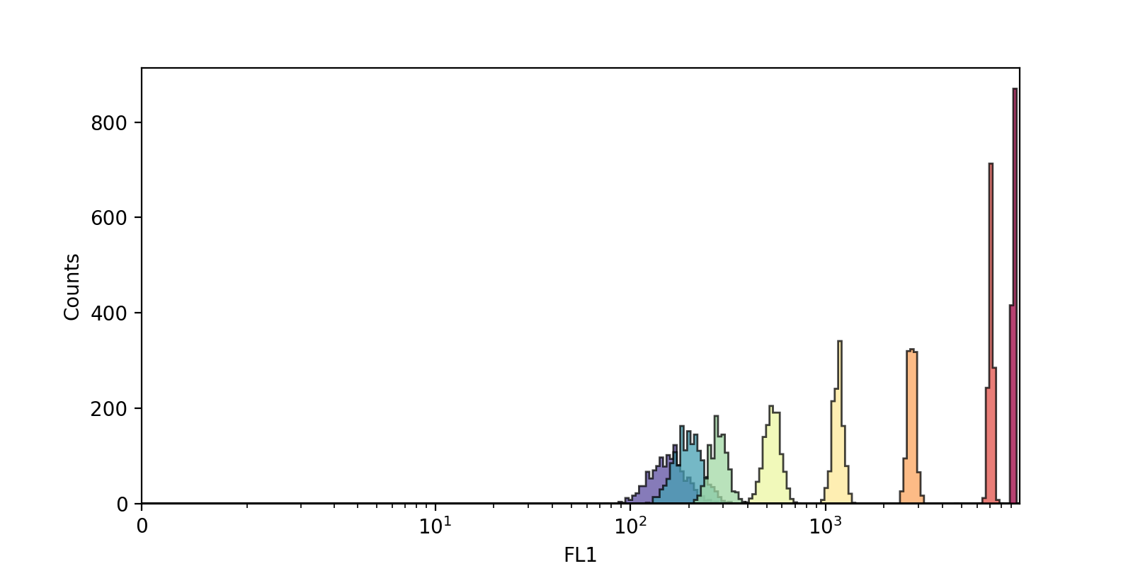
A plot with a default filename of populations_<channel>_<beads_filename>.png is generated by FlowCal.mef.get_transform_fxn() for each channel in mef_channels after the completion of this step. This plot is a histogram showing each population, as identified in step one, with vertical lines showing their representative statistic as calculated from step 2, and with the discarded populations colored in grey. Such plot is shown below, for sample001.fcs and channel FL1.
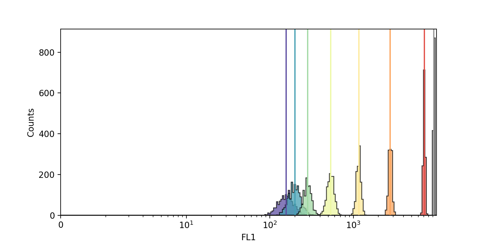
By default, populations whose mean is closer than a few standard deviations from one of the edge values are discarded. This is encoded in the function FlowCal.mef.selection_std(). A different method can be used by providing a different function to FlowCal.mef.get_transform_fxn() through the argument selection_fxn. This argument can even be None, in which case no populations are discarded. Finally, one can manually discard a population by using None as its MEF fluorescence value in mef_values. Discarding populations specified in this way is performed in addition to selection_fxn.
4. Standard Curve Calculation
A bead fluorescence model is fitted to the fluorescence values of each subpopulation in a.u., as calculated in step 2, and in MEF units, as provided in mef_values. A standard curve can then be calculated from the bead fluorescence model.
A plot with a default filename of std_crv_<channel>_<beads_filename>.png is generated by FlowCal.mef.get_transform_fxn() for each channel in mef_channels after the completion of this step. This plot shows the fluorescence values of each population in a.u. and MEF, the fitted bead fluorescence model, and the resulting standard curve. Such plot is shown below, for sample001.fcs and channel FL1.
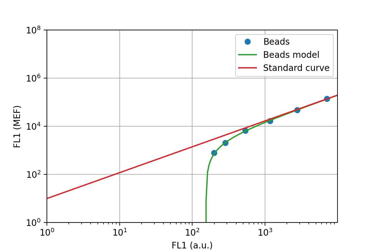
It is worth noting that the bead fluorescence model and the standard curve are different, in that bead fluorescence is also affected by bead autofluorescence, its fluorescence when no fluorophore is present. To obtain the standard curve, autofluorescence is eliminated from the model. Such a model is fitted in FlowCal.mef.fit_beads_autofluorescence(), but a different model can be provided to FlowCal.mef.get_transform_fxn() using the argument fitting_fxn.
After these steps, a transformation function is generated using the standard curve, and returned.
FlowCal.mef.get_transform_fxn() has more customization options. For more information, consult the reference.