Gating Flow Cytometry Data¶

This tutorial focuses on how to gate flow cytometry data using FlowCal, particularly by using the module FlowCal.gate. Gating is the process of retaining events that satisfy some criteria, and discarding the ones that do not.

To start, navigate to the examples directory included with FlowCal, and open a python session therein. Then, import FlowCal as with any other python module.

>>> import FlowCal

Also, import numpy and pyplot from matplotlib

>>> import numpy as np
>>> import matplotlib.pyplot as plt

Removing Saturated Events¶

We’ll start by loading the data from file sample006.fcs into an FCSData object called s. Then, transform all channels into a.u.

>>> s = FlowCal.io.FCSData('FCFiles/sample006.fcs')
>>> s = FlowCal.transform.to_rfi(s)

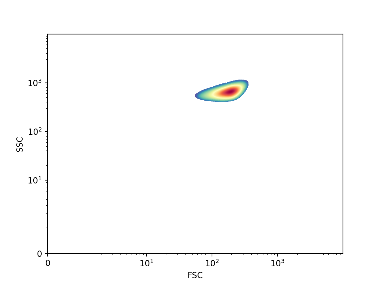
In the plotting tutorial we looked at a density plot of the forward scatter/side scatter (FSC/SSC) channels and identified several clusters of particles (events). This density plot is repeated below for convenience.

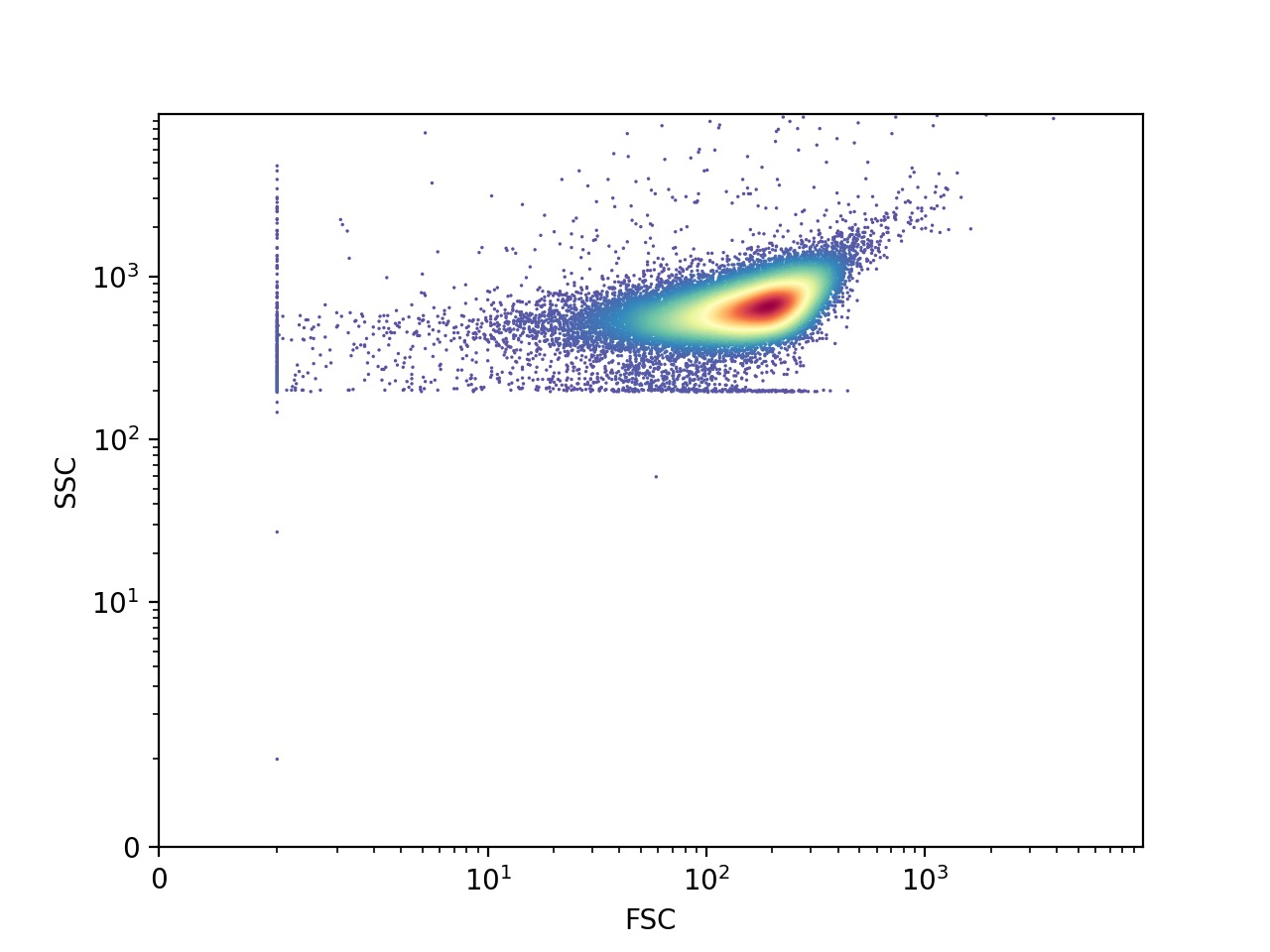
../_images/python_tutorial_plot_density_2d_2.png

From these subpopulations, the faint elongated one in the low-middle portion corresponds to non-cellular debris, and the large one in the middle corresponds to cells. One additional elongated subpopulation on the left corresponds to saturated events, with the lowest possible forward scatter value: 1 a.u..

Some flow cytometers will capture events outside of their range and assign them either the lowest or highest possible values of a channel, depending on which side of the range they fall on. We call these events “saturated”. Including them in the analysis results, most of the time, in distorted distribution shapes and incorrect statistics. Therefore, it is generally advised to remove saturated events. To do so, FlowCal incorporates the function FlowCal.gate.high_low(). This function retains all the events in the specified channels between two specified values: a high and a low threshold. If these values are not specified, however, the function uses the saturating values.

>>> s_g1 = FlowCal.gate.high_low(s, channels=['FSC', 'SSC'])
>>> FlowCal.plot.density2d(s_g1,
...                        channels=['FSC', 'SSC'],
...                        mode='scatter')
>>> plt.show()

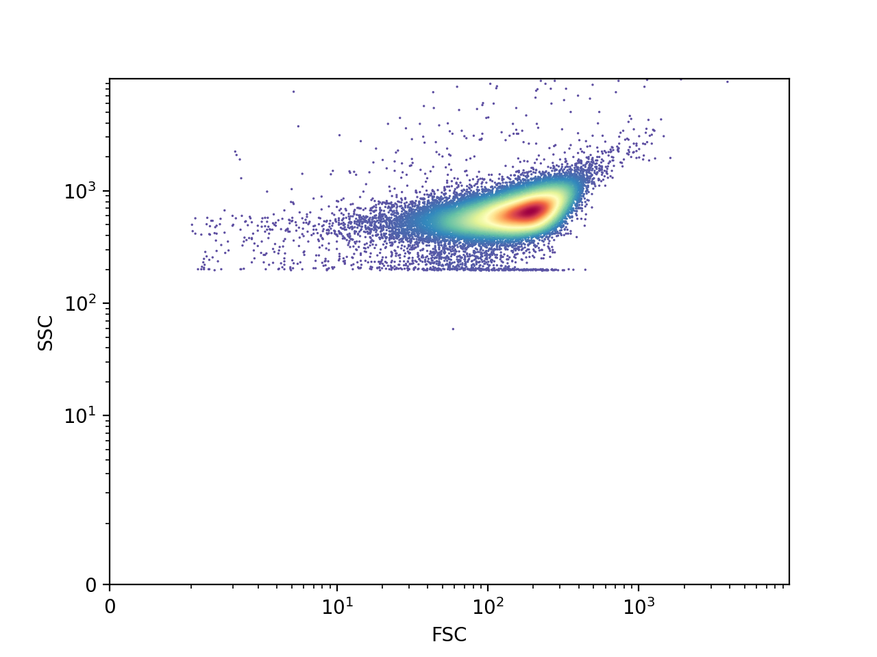
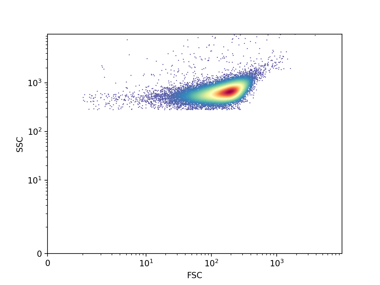
../_images/python_tutorial_gate_high_low_1.png

We successfully removed the events on the left. We can go one step further and use FlowCal.gate.high_low() again to remove some of the events below the main event cluster, which as we said before corresponds to debris.

>>> s_g2 = FlowCal.gate.high_low(s_g1, channels='SSC', low=280)
>>> FlowCal.plot.density2d(s_g2,
...                        channels=['FSC', 'SSC'],
...                        mode='scatter')
>>> plt.show()

../_images/python_tutorial_gate_high_low_2.png

This approach, however, requires one to estimate a low threshold value for every sample manually. In addition, we usually want events in the densest forward scatter/side scatter region, which requires a more complex shape than a pair of thresholds. We will now explore better ways to achieve this.

Ellipse Gate¶

FlowCal includes an ellipse-shaped gate, in which events are retained if they fall inside an ellipse with a specified center and dimensions. Let’s try to obtain the densest region of the cell cluster.

>>> s_g3 = FlowCal.gate.ellipse(s_g1,
...                             channels=['FSC', 'SSC'],
...                             log=True,
...                             center=(2.3, 2.78),
...                             a=0.3,
...                             b=0.2,
...                             theta=30/180.*np.pi)
>>> FlowCal.plot.density2d(s_g3,
...                        channels=['FSC', 'SSC'],
...                        mode='scatter')
>>> plt.show()

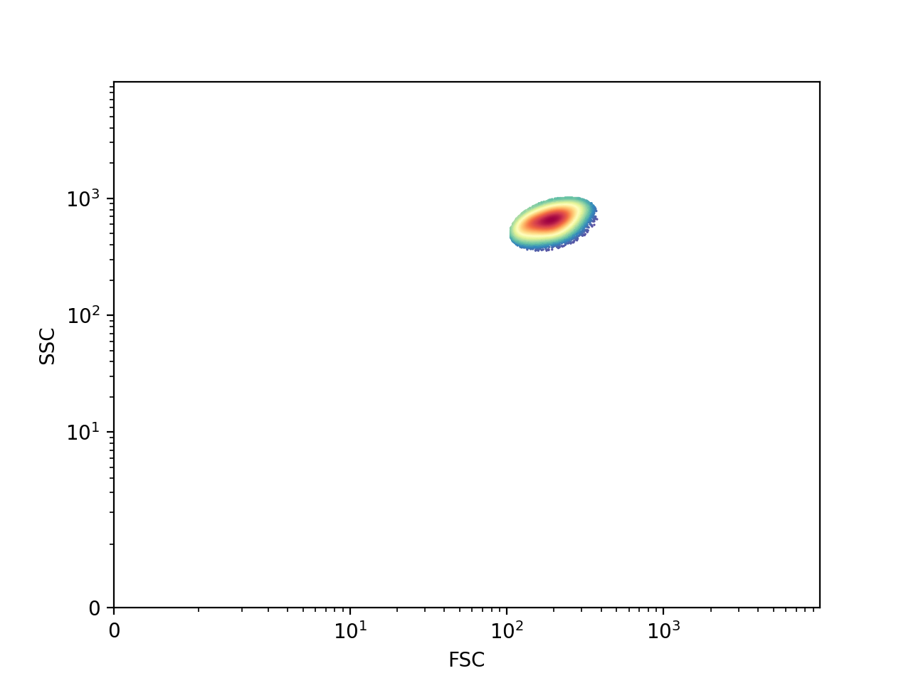
../_images/python_tutorial_gate_ellipse_1.png

As shown above, the remaining events reside only inside an ellipse-shaped region. Note that we used the argument log, which indicates that the gated region should look like an ellipse in a logarithmic plot. This also requires that the center and the major and minor axes (a and b) be specified in log space.

The disadvantage of this gate is that several parameters need to be specified, which make the resulting gate arbitrary. In addition, it is questionable whether we’re actually capturing the densest part of the distribution. Using the mean or median as centers results in similar issues because the original cell distribution is not symmetrical. The next gate solves these issues.

Density Gate¶

FlowCal.gate.density2d() automatically identifies the region with the highest density of events in a two-dimensional diagram, and calculates how big it should be to capture a certain percentage of the total event count. One advantage is that the number of user-defined parameters is reduced to one. Let’s now try to separate cells from debris using this method.

>>> s_g4 = FlowCal.gate.density2d(s_g1,
...                               channels=['FSC', 'SSC'],
...                               gate_fraction=0.75)
>>> FlowCal.plot.density2d(s_g4,
...                        channels=['FSC', 'SSC'],
...                        mode='scatter')
>>> plt.show()

../_images/python_tutorial_gate_density_1.png

We can see that FlowCal.gate.density2d() automatically identified the region that contains cells, and defined a shape that more closely resembles what the ungated density map looks like. The parameter gating_fraction allows the user to control the fraction of events to retain, and it is the only parameter that the user is required to specify.

For more details on how FlowCal.gate.density2d() works, consult the section on fundamentals of density gating.

Plotting 2D Gates¶

Finally, we will see a better way to visualize the result of applying a 2D gate. First, we will use density gating again, but this time we will do it a little differently.

>>> density_gate_output = FlowCal.gate.density2d(s_g1,
...                                              channels=['FSC', 'SSC'],
...                                              gate_fraction=0.75,
...                                              full_output=True)
>>> s_g5    = density_gate_output.gated_data
>>> m_g5    = density_gate_output.mask
>>> contour = density_gate_output.contour

The extra argument, full_output, is available in every function in FlowCal.gate. It instructs a gating function to return additional output arguments with information about the gating process. The second output argument is always a mask (extracted here from the Density2dGateOutput namedtuple using its field name), which is a boolean array that indicates which events from the original FCSData object are being retained by the gate. Two-dimensional gating functions have a third output argument: a contour surrounding the gated region, which we will now use for plotting.

The function FlowCal.plot.density_and_hist() was introduced in the plotting tutorial to produce plots of a single FCSData object. But it can also be used to plot the result of a gating step, showing the data before and after gating, and the gating contour. Let’s use this ability to show the result of the density gating process.

>>> FlowCal.plot.density_and_hist(s_g1,
...                               gated_data=s_g5,
...                               gate_contour=contour,
...                               density_channels=['FSC', 'SSC'],
...                               density_params={'mode':'scatter'},
...                               hist_channels=['FL1'])
>>> plt.tight_layout()
>>> plt.show()

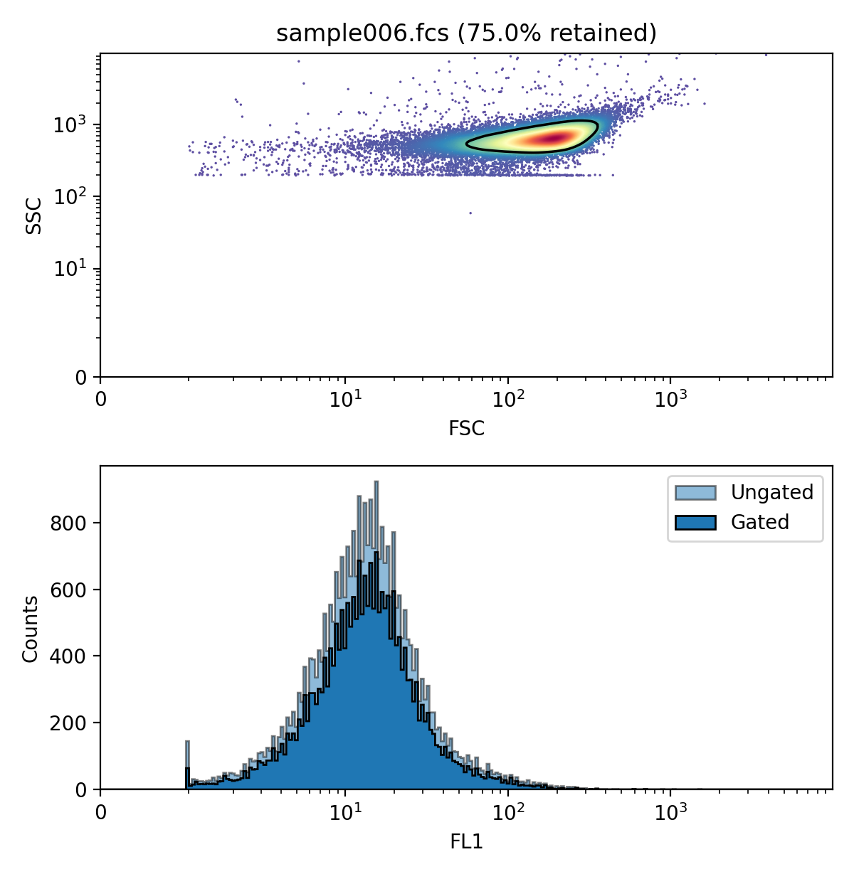
../_images/python_tutorial_gate_density_2.png

We can now observe the gating contour right on top of the ungated data, and see which events were kept and which ones were left out. In addition, we can visualize how gating affected the other channels.